Comparing two places
Two descriptions of San Francisco appear on your screen. One calls a central area expensive, transient and connected. The other calls a western area affluent, settled and isolated. Both sound plausible to someone who already has an image of the city. Neither tells you which people, blocks or years the description covers. An effective comparison begins by taking these apparently simple descriptions apart.
We will compare two actual census tracts using the same statistical release. The exercise is deliberately narrow: two economic indicators can support a description of certain housing and household conditions. They cannot establish the character of residents, the strength of community or the reason someone moved. The challenge is to produce a useful finding while keeping those distinctions visible.
Make the comparison reproducible
Our places are Census Tract 201.01 and Census Tract 353 in San Francisco County, California. Their complete geographic identifiers are 06075020101 and 06075035300. The first lies in central San Francisco; the second lies farther west. These are statistical areas, not claims that a whole named neighborhood has one agreed boundary. The map in chapter one shows their positions using 2024 cartographic boundaries.
The data come from the 2020–2024 American Community Survey five-year release. Five years of responses support estimates for small areas; the release describes that period, rather than a snapshot taken on the final day of 2024. The Census Bureau's comparison of ACS products explains this distinction. Neither tract's value should be presented as its current 2026 condition.
The numbers below were extracted from the official table-based summary files, matched by geographic identifier. Table B19013 supplies median household income; B25064 supplies median gross rent. The 2024 summary-file documentation provides the files and geographic reference. A repeatable comparison records the release, table, variable, geography and units before interpreting the values.
This record does more than help another person reproduce arithmetic. It prevents a familiar mistake: copying a number from one website and another from a different release, then explaining their difference as though only place had changed. When the date, geographic boundary or population differs, part of the apparent contrast may come from the comparison itself.
Read the actual estimates
| Measure | Central tract 201.01 | Western tract 353 |
|---|---|---|
| Median annual household income | $135,759 | $161,074 |
| Published 90% margin of error | ±$34,324 | ±$32,675 |
| Median monthly gross rent | $2,821 | $3,469 |
| Published 90% margin of error | ±$385 | ±$459 |
Values are in 2024 dollars. Income is the household measure specified in B19013's variable definitions, not each individual's wage. Gross rent combines contract rent with applicable estimated utility and fuel costs; the median excludes units with no cash rent. Its universe is renter-occupied housing paying cash rent, rather than every household. See the gross-rent section of the 2024 ACS subject definitions.
Those differences in population matter. A large income estimate for all households does not tell us that the typical renter receives that amount. Owner households and renter households may have different incomes. A household may also contain several earners. Converting the income median into a supposed individual salary would change the measure without changing its label.
The rent values describe occupied rental housing in the survey's defined population. They are not advertised prices for newly available apartments, prices per bedroom or quotations for identical homes. A tract with more large rental homes could have a higher median even if a comparable small unit did not cost more. We have not measured that composition here.
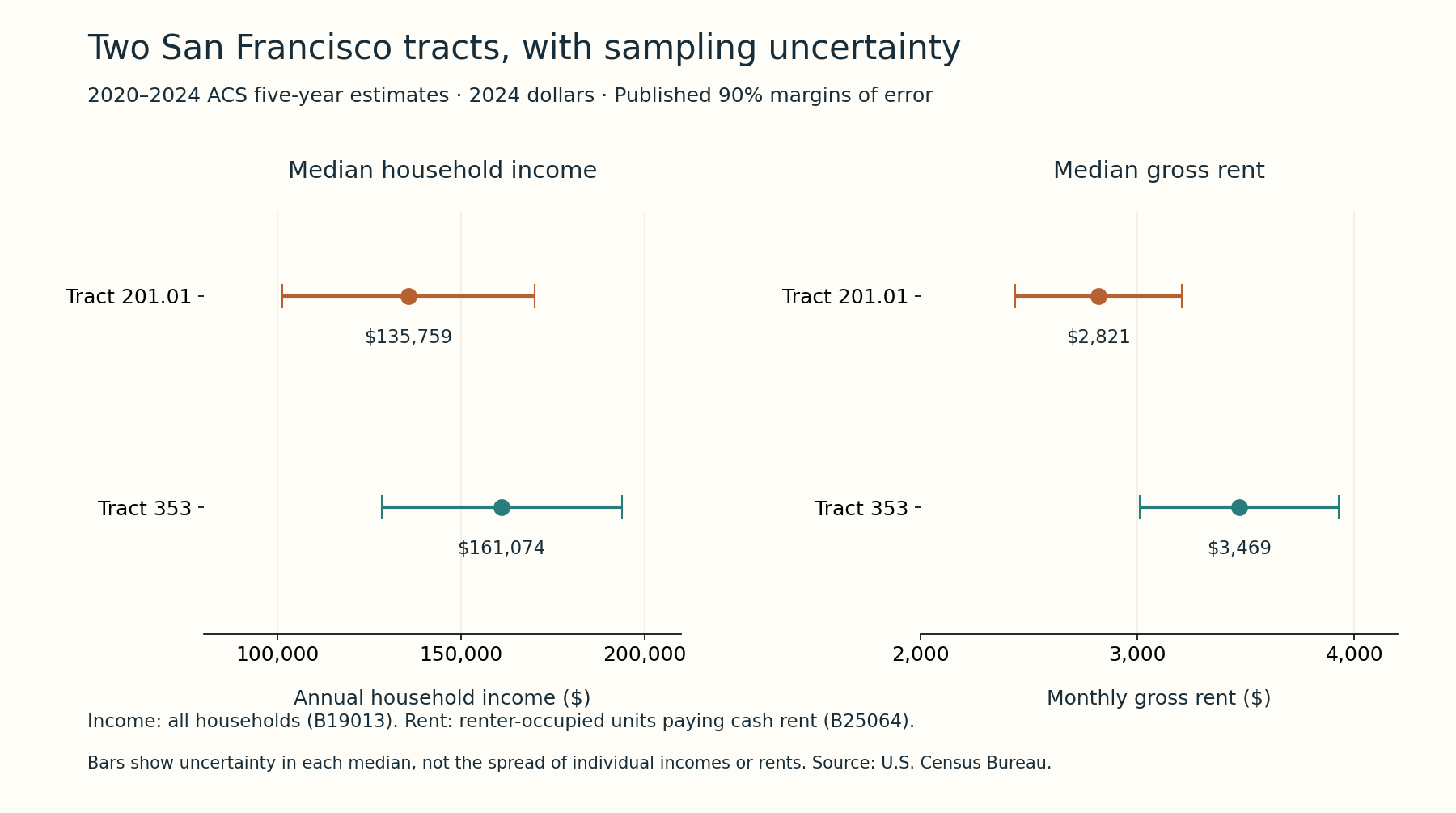
Original chart from the 2020–2024 ACS five-year summary files. Income and rent use different populations and time units. Bars describe sampling uncertainty around each estimate, not the range of household incomes or rents.
What uncertainty changes
A sample estimate is not an exact census of every value in the population. The published margin of error helps express sampling uncertainty. Under the ACS convention, adding and subtracting the margin produces a 90% confidence interval. The interpretation concerns the repeated performance of the estimation procedure, not a statement that 90% of households fall inside the interval. Margins do not capture every possible source of error. These conventions are documented in ACS Accuracy of the Data.
For central tract income, subtraction and addition give $101,435 to $170,083. For western tract income, they give $128,399 to $193,749. The point estimates differ by $25,315, yet each estimate has substantial uncertainty. It would be misleading to display the point values to the dollar and describe the relative position as precisely established.
We can examine the difference directly. Using the Census statistical-testing approximation, which omits covariance between the two estimates, the margin for a difference is the square root of the sum of their squared margins. For income, that is approximately $47,390. The difference of $25,315 therefore has an approximate 90% interval from −$22,075 to $72,705. Zero lies inside it: this calculation does not establish a positive income difference at that confidence level.
Failure to establish the direction is not proof that the underlying medians are identical. The range also accommodates economically substantial differences. A useful report gives the estimate and uncertainty rather than replacing an uncertain result with an assertion of equality. Precision is part of what the study found, including when the available sample cannot answer the question sharply.
For rent, the individual intervals are $2,436–$3,206 and $3,010–$3,928. Their overlap might tempt a reader to declare the difference statistically inconclusive. But overlapping individual intervals are not the correct test of the difference. Under the same approximation, the difference is $648 with a margin of about $599: an interval of roughly $49–$1,247, above zero at 90% confidence.
This example shows why an interval is preferable to a ranking alone. The rent comparison supports a positive difference under the stated method, but its size remains uncertain. It does not establish a difference for identical apartments, nor a cause. The Census Bureau's statistical testing guidance is an appropriate starting point for further comparisons. Overlapping geographies or estimates from overlapping periods require particular care about dependence; our simple calculation should not be copied automatically into those settings.
There is another decision to record: why these two places and these two indicators were selected. They provide a manageable teaching comparison, not a representative sample of all San Francisco neighborhoods. Searching hundreds of tract pairs and reporting only the largest or most statistically striking contrast would change the interpretation of the test. A reader needs to know whether a comparison was chosen to answer a prior question or discovered while exploring many possibilities. Exploratory work is useful when it is identified as such.
Do not manufacture an affordability measure
A tempting next step divides twelve times median rent by median household income. The arithmetic produces a tidy percentage, which can easily acquire the label “typical housing burden.” But chapter two showed why a ratio of separate medians is not the median of household ratios. Here the populations also differ: income covers all households while rent covers a particular rental universe.
A valid rent-burden analysis needs a measure that relates housing costs to the incomes of the households paying them. It also needs a stated treatment of households for which a ratio cannot be calculated. A different table may supply an appropriate distribution, but its existence does not license us to invent the result from the two medians already on hand.
Imagine two households paying the same $3,000 monthly rent. One has $4,000 monthly income; the other has $12,000. Their burdens are 75% and 25%. Averaging rent across them loses none of its variation because there is none, but averaging income would produce a ratio of 37.5%. That number describes neither household. Aggregation can conceal the exact mismatch that made affordability the question.
Nor does a lower rent median necessarily make a place more accessible to a new entrant. Existing tenancy terms, scarce vacancies, home size, deposits and application requirements can intervene. An access claim requires evidence about the route into housing. A cost distribution among current occupants answers a related question, with a different population selected by past entry and exit.
Add evidence without pretending it is interchangeable
Our table cannot describe public life. We could add observations using chapter four's protocol: fixed locations, matched durations and recorded weather, events, entrances and seating. Such observations would reveal use at those times. They would not give a representative account of every resident's friendships or establish why a person chose to sit alone.
We could also add a public planning document. It might establish a property's designated use, a recorded decision or a project's stated intention. It would not automatically establish implementation or its effects. A hearing record can reveal arguments that participants presented; it cannot silently substitute for a survey of all residents. Each additional source needs a sentence stating what it can support.
Consider an explicitly hypothetical extension: one tract contains a plaza where twelve people are present during an evening observation, and the other contains a plaza with three. Even if the counts are accurate, the areas could differ in plaza size, accessible entrances, weather exposure or events. The observation does not validate the original labels “connected” and “isolated.” It creates a narrower question about use of these spaces under specified conditions.
History introduces another kind of evidence. A documented clearance project can explain how certain buildings disappeared and why households faced relocation. It does not by itself identify the entire cause of a modern tract's income distribution. Connecting past intervention to a present outcome requires intermediate evidence about later construction, occupancy, movement and resources. A vivid event can be causally important without being a complete explanation.
Build two explanations that can lose
Suppose your question becomes: why is estimated gross rent higher in tract 353 than in tract 201.01 during this period? One explanation emphasizes the composition of rental homes. It predicts that differences in size or type account for part of the contrast. A second emphasizes differences in tenancy duration and the terms faced by existing occupants. It predicts a contrast associated with those features even among homes of comparable type.
These are hypotheses, not findings from our two tables. To distinguish them, you would need evidence measuring the proposed mechanisms. Matching similar homes might help with composition but would not automatically remove selection into tenancy. A model with many controls can still miss relevant differences. The correct next step is to specify the evidence needed, rather than to add a confident causal sentence after the descriptive chart.
A third explanation could emphasize location-related demand. Again, a useful version must say what makes the location desirable to whom and how that demand reaches observed rents. Access to jobs, schools or amenities cannot all be represented by a vague label such as “better neighborhood.” Different households value different bundles and face different constraints. An explanation becomes testable when its mechanism has observable implications.
Strong comparisons also admit that several mechanisms may operate together. Their task is not necessarily to choose one exclusive winner. It may be to determine which mechanisms matter, for which households, under which conditions. Rejecting a single-cause story does not mean every proposed explanation receives equal support.
The objection: is this too cautious to be useful?
An impatient reader might prefer a clear ranking and a recommendation about where to live. Our analysis cannot responsibly provide that recommendation, because it lacks the person's needs and the relevant current housing options. But it already supplies useful conclusions: the places and period are explicit, the rent difference has been evaluated, the income ranking is uncertain, and several common interpretations have been ruled out.
That is progress over an impression dressed as data. It also directs further work. A housing question calls for information about comparable homes, occupants and entry. A community question calls for evidence about relationships and institutions. A public-space question calls for observations designed around access and use. The available indicator should not choose the question merely because it is easy to download.
The final comparison should preserve a distinction between describing conditions and judging them. You may value affordability, continuity, mobility, diversity or quiet. State those priorities and acknowledge tensions among them. A finding about median rent cannot decide how to weigh an incumbent's security against another household's opportunity to move in. Empirical discipline makes the disagreement clearer; it does not remove the need for judgment.
Check your understanding: The two tracts have overlapping individual rent confidence intervals. Must their difference be statistically inconclusive, and can their rent-to-income median ratios measure typical rent burden?
Expected answer: Neither inference follows. Test the difference using its uncertainty; the stated approximation gives a positive rent difference at 90% confidence. Ratios of separate medians do not give a median household burden, and these rent and income figures have different populations.
Application
Write a 1,000–1,500-word comparison of these two tracts, or two places for which you can obtain equivalent evidence. Allow about two hours for assembly and writing, in addition to the earlier chapter exercises.
Include a map with explicit boundaries; a dated table or chart with units, populations and uncertainty; one observation record or clearly labeled use of the supplied fictional plaza case; and one historical or institutional source whose limits you explain. If you do not visit the places, say so. Do not transplant the Western Addition history into either tract without checking the geographic connection.
Develop two explanations for one defined contrast. Identify the evidence that would discriminate between them and one result that would weaken your preferred explanation. Separate findings, hypotheses and values in the prose rather than hiding every qualification in an appendix.
A successful submission can be reproduced, avoids describing people through tract averages, and makes a modest claim that its evidence actually supports. A weak submission offers a neighborhood ranking without comparable data. Before finishing, ask someone to identify your population, period and causal claim from the opening paragraph; revise if those remain unclear.