Comparing explanations and responses

A fictional policy committee asks for a brief on household income and inequality. Its members want to know why some places have higher incomes, whether moving families would improve opportunity and what evidence could justify spending public funds. One member arrives with a state ranking, another with a memorable family story and a third with a research paper. The task is to make these materials answer precise questions instead of letting each support whatever conclusion its presenter already prefers.

Our final chapter supplies a small, dated dataset and a housing experiment. The dataset describes places; the experiment tests an intervention for a particular population. Neither chooses the committee's values or settles every mechanism. Your task is to use them together without confusing description, causal inference and judgment.

Begin with a reproducible description

The table below reproduces selected 2023 ACS one-year estimates from the Census Bureau's September 2024 income brief. It reports household income and an income Gini, with 90-percent margins of error. These are four selected states plus a national reference, not a representative sample of states or a current-2026 ranking. Census brief, Table 1.

Geography	Median household income, 2023 dollars	90% margin	Income Gini	90% margin
United States	$77,719	±$186	0.483	±0.001
Alaska	$86,631	±$2,575	0.449	±0.012
California	$95,521	±$611	0.487	±0.002
Massachusetts	$99,858	±$1,355	0.488	±0.004
New Jersey	$99,781	±$1,061	0.479	±0.004

The unit is the household, not an individual worker. The survey asks about the preceding twelve months, and national inflation adjustment does not equal adjustment for local living costs. The definitions and measurement issues established in chapter one continue to apply. A concise description can refer back to them while retaining the population, vintage and units beside the numbers.

A reproducible account identifies the exact table and selected rows, preserves the margins and explains any transformations. Here, the original chart converts dollar amounts to thousands only for its horizontal axis. It does not change the estimates or remove observations. Someone following the stated source and calculation should be able to recover the displayed values.

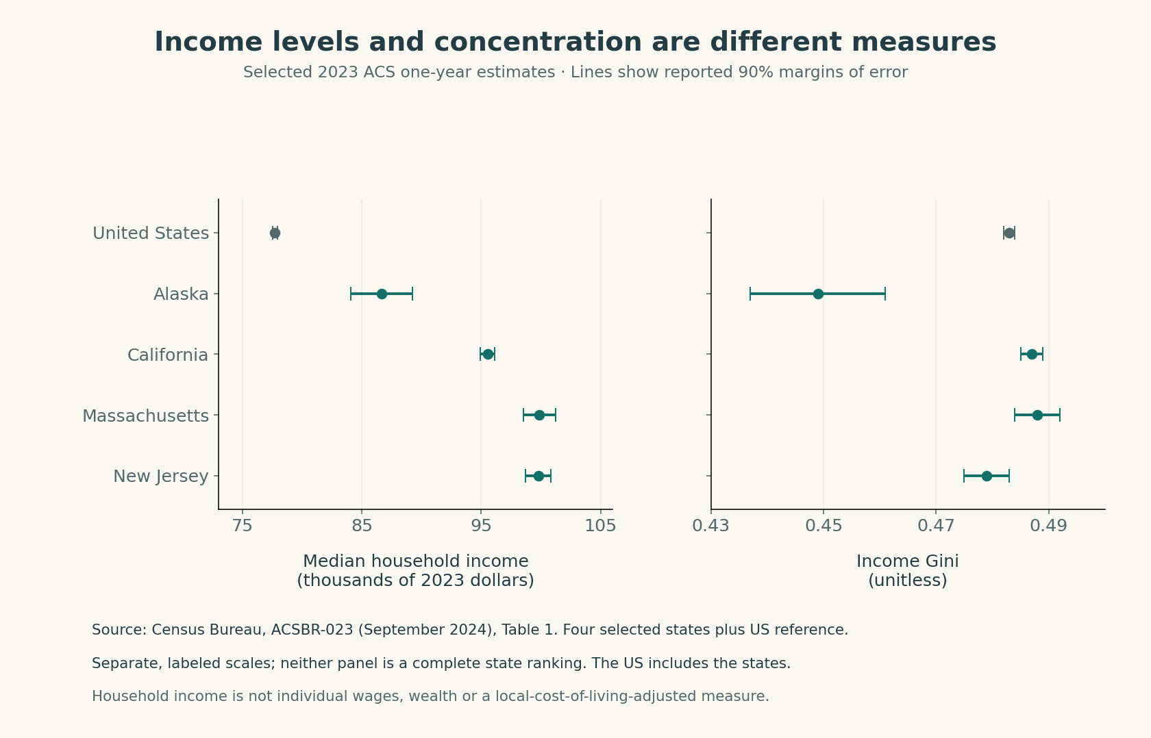
A rank is less certain than its printed order suggests

Massachusetts has a point estimate seventy-seven dollars above New Jersey. Their margins of error are much larger than that difference. The Census report explicitly identifies these state estimates among those not statistically different. A brief should not turn their printed order into evidence that one state's households have decisively greater resources than the other's.

The individual income intervals are straightforward to calculate. Massachusetts spans 98,503 to 101,213 dollars; New Jersey spans 98,720 to 100,842. These intervals describe uncertainty under the survey procedure. They do not mean that ninety percent of households have incomes inside the interval, and they do not describe the spread of incomes within either state.

Overlap is a visual cue, not a universal hypothesis test. Comparing two estimates formally requires the uncertainty of their difference and any relevant covariance. The national estimate also contains households from the states, so treating national and state estimates as independent observations would be inappropriate. In this exercise, use the published report's comparison where available and avoid inventing precision beyond it.

The Gini panel answers another question. California and New Jersey have different point estimates of concentration even though both have relatively high median incomes among the selected rows. We should describe the specific estimates and their uncertainty rather than infer a universal relationship from four states. A higher median does not mathematically require a lower or higher Gini.

Chart choices should expose the comparison

The two panels use separate axes because dollars and Gini values have different units. Each panel is a point-and-interval plot: the point marks the estimate and the line marks the reported margin. The income axis is explicitly labeled in thousands of dollars, while the Gini axis is unitless. The chart does not use bar lengths to imply that a small truncated range begins at zero.

This choice makes uncertainty visible without filling the page with duplicate figures. The table remains available for exact values. A reader should be able to tell which differences are large relative to the displayed intervals and which printed ranks deserve caution. The visual supports the reasoning instead of substituting color or height for a defined measure.

Selection also belongs in the caption. We chose these rows to illustrate differences in levels, concentration and uncertainty, not because they prove a favored policy. Omitting that fact could make the chart look like a complete national comparison. A small teaching dataset is useful when its boundaries are explicit.

Do not add a fitted causal line through these five points. The national reference is not another independent state, the four states were selected, and the table contains no design that isolates a policy effect. A line might summarize the chosen coordinates mathematically, but it would not establish why incomes or inequality differ.

Move from a pattern to competing mechanisms

Suppose the committee asks why California's median exceeds the national median in this dataset. One possible mechanism concerns the mix of jobs and industries. Another concerns which households live in the state and how many earners they contain. Differences in education, migration, hours, prices and other institutions may also matter. The table itself does not distinguish among these accounts.

To develop the job-composition explanation, specify a sequence: the local distribution of employment opportunities affects access to occupations and their rewards, which contributes to household income. Evidence would need to connect those stages. A simple count of high-paying industries would not show that every household benefits or that the industry mix caused the observed median.

For a household-composition explanation, investigate the number of earners, ages and household sizes under consistent definitions. A higher household median might partly reflect more earners per household without a corresponding increase in each individual's wage. That possibility does not make the household estimate wrong. It changes what additional measures are needed to interpret it.

A serious alternative should be capable of changing the conclusion. Merely writing “other factors may matter” does not do this. State what the alternative predicts and what evidence would favor it. If an apparent difference becomes much smaller under a relevant composition comparison, that would affect an account based entirely on higher rewards for otherwise similar work. The adjusted comparison would still need its own assumptions explained.

A housing experiment asks a different question

Moving to Opportunity randomly offered housing assistance to 4,604 families in five US cities during 1994–1998. Its experimental arm combined a voucher initially restricted to low-poverty neighborhoods with mobility counseling; another arm offered a regular voucher, and a control group received no MTO offer. The assigned reading is the authors' August 2015 version of a study later published in 2016. Author-hosted paper; publication record.

The study links participants to later records and reports improved adult economic outcomes for children who were younger when their families received the experimental offer, with different results for older children and adults. Assignment was to an offer, not to a completed move. The intervention changed access to a bundle of conditions; it did not isolate one neighborhood feature or establish a universal age threshold.

This is a different evidential object from our state table. Random assignment supports a comparison between groups offered different assistance under the study's design. It does not answer what would happen if any household moved from any lower-income state to a higher-income state. The population, intervention, destination conditions and historical context are specific.

The age pattern also requires care. It may be consistent with differing exposure or disruption, but those interpretations are not identical to the randomized offer comparison. We should distinguish the estimated consequence of the intervention from explanations for why its effects vary. A persuasive mechanism needs evidence beyond naming a plausible story after seeing the result.

The effect of an offer differs from the effect of taking it up

Consider a separate invented experiment with one hundred families assigned an offer and one hundred assigned no offer. Suppose half of those offered assistance use it. A comparison of all assigned families preserves the original assignment. Comparing only the fifty users with the controls does not, because users may differ from nonusers in motivation, constraints or expected benefit.

An intention-to-treat estimate describes the effect of assignment to the offer. In the invented example, suppose the average later outcome is 1,000 units higher in the offer group. Under additional assumptions, an instrumental-variable calculation might scale that by the fifty-percentage-point difference in take-up, yielding 2,000 units for a particular group whose participation changes because of the offer.

Those additional assumptions matter. They include how assignment affects outcomes beyond participation, whether the comparison actually changes participation as stated and whether the relevant response pattern is appropriate for the interpretation. The scaled result is not automatically the effect for every person who could ever move. We use round invented numbers here to explain the distinction, not to reproduce the MTO estimates.

For a decision-maker offering a real program, the offer effect can itself be highly relevant. It includes the fact that some eligible families cannot or do not use the assistance. Low take-up may indicate an implementation obstacle or a reasonable choice under particular circumstances. Excluding nonusers from the headline does not solve that practical problem.

An intervention effect does not identify every mechanism

Imagine that a voucher changes housing quality, travel, school access, social contacts and exposure to disruption. A favorable outcome for the offered group does not reveal which component mattered most. Nor does it show that changing only one component would reproduce the effect. The intervention is a package, and its internal pathways may interact.

Mechanism evidence could examine timing, intermediate outcomes and variation relevant to a specific account. If a proposed explanation depends on access to an activity, establish whether access actually changed. If it depends on reduced disruption, investigate the sequence of moves and experiences. Such evidence can strengthen an interpretation while requiring caution about comparisons no longer protected by the original random assignment.

Transportability is another question. A new program may operate where housing supply, available destinations, services or participant needs differ. The historical experiment provides evidence worth using, but a responsible proposal identifies which conditions must hold for the mechanism to work in the new setting. Similar labels do not guarantee equivalent interventions.

This is where the state chart could otherwise mislead. A higher state median is not a treatment that can be administered to a family. Moving to a state changes a particular household's circumstances, not its income mechanically to the state's median. Inferring an individual's expected gain from the difference between place averages confuses population composition with an intervention.

Values enter when we compare responses

Suppose the committee considers relocation assistance, support for existing neighborhoods or direct financial help. Each proposal can pursue a different objective and operate through different pathways. A useful comparison states the intended beneficiaries, costs, timing, likely mechanisms and outcomes that would count as success. It should also explain which tradeoffs the committee is willing to accept.

One standard might prioritize improving the prospects of children facing severe constraints. Another might emphasize preserving valued local relationships or allowing adults greater choice. A third might focus on the largest measured gain per unit of public spending. Evidence can reveal consequences and tensions among these standards, but it cannot select the ethical weights without an argument.

The distribution of benefits and burdens matters. An average gain can coexist with losses for a subgroup or costs imposed on people outside the study population. Conversely, a policy serving a disadvantaged group should not be dismissed merely because it does not improve every outcome for everyone. The evaluation needs a stated objective and a serious account of relevant consequences.

Your final brief should therefore make a bounded recommendation. Explain what you would do under the available evidence, what remains uncertain and what observation would lead you to revise the proposal. This is stronger than either claiming certainty or refusing to decide until every question is answered. A responsible judgment connects evidence, assumptions and values so that another reader can examine each part.

A sensitivity analysis can make the recommendation more useful. In a wholly invented budget exercise, suppose an offer costs 2,000 units per eligible family and yields a benefit the committee values at either 1,000, 3,000 or 5,000 units under three plausible scenarios. The corresponding net values are negative 1,000, positive 1,000 and positive 3,000. The decision turns partly on which scenario is credible and whether the stated valuation captures the objective. This arithmetic is not an appraisal of MTO; it demonstrates how to reveal a threshold rather than hide uncertainty inside a single favorable estimate.

You can then ask what additional information is worth obtaining. If modest changes in an uncertain assumption reverse the recommendation, a pilot or better measurement may be valuable. If the conclusion remains stable across the relevant range, further precision may be less decisive. The point is to connect uncertainty to the decision it could change, while keeping unpriced values and distributional concerns visible.

Application

Write a 1,200–1,600-word inequality brief for the fictional committee. Use the supplied ACS table to make one accurate descriptive comparison and include your own chart or a clearly attributed use of the course chart. State the dataset vintage, household population, units, selected-geography limits and margins of error. Develop two mechanisms and a serious alternative; identify evidence that would distinguish them. Use the housing study to explain the difference between a place comparison and a randomized offer. Finish with a bounded policy recommendation and an explicit normative standard.

Evaluation guide: A strong brief keeps dollar levels separate from concentration, preserves uncertainty, avoids treating state averages as individual treatment effects, distinguishes offer from take-up, and makes the proposed causal sequence inspectable. It uses an alternative that could change the conclusion and names an outcome that could challenge the recommendation. A weak brief ranks the states as an all-purpose measure of well-being, treats overlapping estimates as exact ranks, or attaches a policy claim to the table without an identification argument.

Check your understanding: Can the difference between California's median and the national median estimate how much a family would gain by moving to California, and does a randomized voucher offer identify the effect of every completed move?

Expected answer: No. The median comparison describes different household populations and does not isolate a relocation effect. Random assignment identifies an offer comparison under the study's design; completed moves involve take-up, and estimating participation effects requires further assumptions. A recommendation must match its evidence to the actual population, intervention and objective.