Timing the beat

Imagine two mechanical pumps receiving an instruction every eight tenths of a second. One has an unobstructed outlet and a chamber full of liquid. The other has an outlet that cannot open. Their instruction logs could look identical while their deliveries differ completely. Counting commands would tell us something valuable about timing, but it would not tell us how much liquid moved.

An electrical recording of the heart poses a related problem. Electrical activation helps initiate contraction, but activation, force, pressure, and flow are different events. The challenge in this chapter is to connect them without turning them into synonyms. We need three maps: one of a cell's changing voltage, one of excitation spreading through tissue, and one of the signal measured at the body surface.

A clock made of living cells

The sinoatrial node, usually shortened to SA node, contains specialized cardiac cells that normally establish the heart's rhythm. It lies in the right atrium near the entrance of the superior vena cava. Its cells can generate repeated electrical activity without receiving a separate command from the brain for every beat. This capacity is called automaticity. Nervous and hormonal influences can change the rhythm; they do not have to manufacture every initiating event. University of Minnesota: conduction overview.

A cell's membrane potential is the electrical potential difference across its membrane. When that difference becomes less negative inside, we call the change depolarization. Repolarization restores a more negative membrane potential. An action potential is a coordinated excursion in this voltage, produced by changing ion movements through membrane channels.

In pacemaker cells, the voltage does not remain at a stable resting level between successive action potentials. Interacting ion currents bring it toward another activation. Calcium currents contribute prominently to the rising phase, while potassium currents contribute to recovery. These are regulated membrane processes, not a tiny metal wire repeatedly touched to a battery. Their rates can change. Klabunde: sinoatrial action potentials.

Consider what the clock analogy gets right. An oscillator supplies recurring events, and changing its period changes how frequently they occur. Now consider what it leaves out. A living oscillator depends on membrane channels, ion gradients, metabolism, and surrounding tissue. Its period is adjustable, and the cells participating in the rhythm interact. The analogy helps us ask about repetition; it does not explain the mechanism by itself.

Passing excitation onward

Most working ventricular muscle cells normally respond to excitation arriving from other cells. Their action potentials have a rapid rising phase and a prolonged plateau before recovery. Sodium, calcium, and potassium currents contribute at different stages. During an effective refractory period, recently activated tissue cannot produce another normally propagated response. Recovery therefore constrains how soon the next effective excitation can pass. Klabunde: non-pacemaker action potentials.

The plateau is not the same thing as an ECG line staying above its baseline. One describes voltage across an individual cell membrane; the other is a measurement made outside many cells. Keeping those measurement locations separate will matter shortly.

Adjacent cardiac cells communicate electrically through gap junctions, channels connecting their interiors. Current flowing through these connections helps bring neighboring cells to activation. The wave advances because new cells generate their own response. Tissue arrangement, cellular electrical properties, and coupling affect how quickly excitation spreads. The AV nodal region conducts relatively slowly; the downstream ventricular conducting network distributes excitation rapidly. University of Minnesota: cell-to-cell conduction.

Draw five connected circles on paper. Label them A through E. Initially only A is activated. Next, B activates while A is recovering; then C activates while B follows A into recovery. The moving boundary of newly activated cells differs from the set of cells that have already responded. A snapshot showing three changed circles cannot, by itself, identify the speed or direction of the boundary. You need another snapshot or a record of their activation times.

This small model explains why a conduction map should contain arrows and timing information, not just colored tissue. It also shows why recovery matters. The immediately preceding region is not automatically ready for another identical response. A realistic account must track both where excitation can go and which tissue can respond when it arrives.

A sequence with a deliberate delay

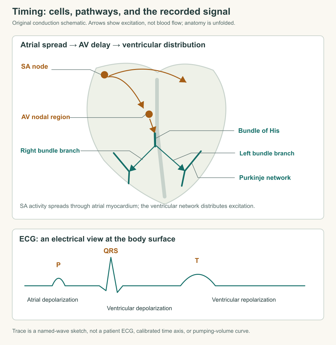
The usual route begins with excitation spreading through the atria from the SA nodal region. It reaches the atrioventricular, or AV, nodal region and then the bundle of His. The pathway continues into right and left bundle branches and the Purkinje network, which distributes excitation to ventricular muscle. The atrial spread should not be imagined as three perfectly isolated insulated cables: the organization includes connected myocardium and preferential routes. University of Minnesota: conduction overview.

Why slow transmission on the way to the ventricles and then distribute it rapidly within them? The tasks differ. A delay between atrial and ventricular activation helps preserve their sequence. Rapid distribution within the ventricles helps organize their contraction. Most ventricular filling does not wait for atrial contraction, as the previous chapter showed, but the timing of atrial contribution still matters.

An original timing model makes the distinction precise. Assign three successive stages transmission times of 20, 90, and 30 milliseconds. These are invented values for a teaching network, not reference measurements of named human structures. The total delay from input to output is 140 milliseconds. If the input occurs every 800 milliseconds and every input passes through, the output also recurs every 800 milliseconds, simply displaced later in time.

Now shorten the middle stage to 60 milliseconds. Output arrives after 110 milliseconds instead of 140. Has the repeating rate increased? No. Each output comes earlier relative to its input, but adjacent outputs remain 800 milliseconds apart. Transmission delay and repetition period answer different questions.

Alternatively, retain the original 140-millisecond delay but supply inputs every 600 milliseconds. Outputs now recur every 600 milliseconds, provided the network can still respond to each input. We changed the clock without changing the assigned travel time. In living tissue, these properties can interact; separating them first lets us recognize an interaction instead of assuming one.

What the surface recording measures

An electrocardiogram, or ECG, records differences in electrical potential at the body surface. Its signal reflects the combined activity and activation sequence of many cells, modified by their arrangement, the surrounding tissues, and the recording locations. It is neither a photograph of the chambers nor the action potential of one representative cell. Noble, Hillis, and Rothbaum: electrocardiography.

An electrode is a physical sensor. A lead is an electrical view defined by a particular comparison of potentials. Different views of the same cardiac event can produce different waveforms. A downward deflection does not mean the heart pumped backward, just as an upward deflection does not measure upward blood movement. Direction and sign belong to the specified electrical measurement. Noble, Hillis, and Rothbaum: electrocardiography.

Take a purely mathematical example. At one instant, imagine the measured potential at location A is 0.3 arbitrary units and at B is 0.1. Reporting A minus B gives +0.2. Reversing the comparison gives −0.2. Nothing in the source changed. Only the reporting convention changed. Real ECG leads involve a defined electrode arrangement, but this subtraction captures why the sign requires a reference.

There is another implication. Suppose two contributions to a selected measurement are +0.4 and −0.4 units. Their sum is zero despite neither contribution being zero. This invented cancellation example is not a model of two anatomical chambers. It demonstrates a general property of combined signals: a small net measurement need not mean that all contributing processes are small or absent.

Reading the names without overreading them

In a typical schematic ECG, the P wave represents atrial depolarization. The QRS complex represents ventricular depolarization, and the T wave represents ventricular repolarization. Atrial repolarization is usually obscured by the larger ventricular signal. The PR interval runs from the beginning of P to the beginning of QRS: it includes more than a pure stopwatch measurement of AV nodal delay. Klabunde: the ECG.

These names locate electrical events. They do not label the quantities “blood entering,” “blood leaving,” and “blood returning.” To discover whether a ventricle is ejecting at a particular time, we still need the mechanical relationships developed in Chapter 3: chamber pressure, outlet pressure, valve state, and changing chamber volume.

The relatively level ST segment of a schematic recording lies between ventricular depolarization and the main repolarization wave. Much ventricular tissue is still in its depolarized phase during this interval. A level segment therefore does not imply that all ventricular cells have returned to their resting state. Klabunde: the ECG.

Imagine placing three transparent sheets over one another. The first carries an ECG, the second ventricular pressure, and the third ventricular volume. Their horizontal axes all represent the same time. Each sheet answers a different question. Aligning them helps explain the sequence; replacing the pressure and volume sheets with copied ECG curves destroys the explanation. Matching timestamps do not make different measurements interchangeable.

There is a practical way to test whether your three-sheet explanation makes sense. Hide two sheets and list exactly what remains observable on the third. With only the volume sheet, you can identify intervals of increasing, decreasing, or approximately constant chamber volume. You cannot directly label the membrane voltage of a particular cell. With only the electrical sheet, you can identify the timing of its recorded waveforms, but you cannot calculate the difference between end-diastolic and end-systolic volumes. With only the pressure sheet, an isolated value still needs a comparison with pressures across the relevant valve. Restoring the other sheets supplies missing relationships. It does not retroactively turn any single sheet into a complete measurement of the heart. This exercise makes the boundary of each inference visible before you start naming abnormalities.

Counting intervals correctly

Suppose a supplied record marks successive ventricular electrical events at 0, 0.8, 1.6, 2.4, and 3.2 seconds. There are five marks, but only four completed intervals between the first and last. Each interval lasts 0.8 seconds. The repetition rate is therefore 60 ÷ 0.8 = 75 events per minute.

Counting five marks and dividing by 3.2 seconds would give 93.75 per minute. That calculation mishandles the endpoints: the event at zero begins the first interval rather than completing an extra one within the measured span. Counting events in a separately defined fixed window is another method, with its own boundary convention. Here we are deliberately using the elapsed time between marked events.

Now alternate intervals of 0.6 and 1.0 seconds. Two completed intervals occupy 1.6 seconds, so the overall rate across each pair is again 75 per minute. The interval-specific rates are 100 and 60 per minute. Their ordinary arithmetic mean is 80, which differs from the overall rate because the slower interval occupies more time. Dividing completed intervals by total elapsed time preserves that weighting.

The two records consequently share an overall rate while differing in regularity. A single average cannot describe everything about a rhythm. A useful description identifies the interval distribution as well as the summary number. This is a mathematical lesson about the supplied records, not a classification of someone's health.

Matching evidence to a question

Surface electrodes record the heart's existing electrical signals; an ordinary ECG does not send electricity into the body. A short recording also samples only a short period. An event absent from that sample may occur outside it. These limitations help explain both the usefulness of electrical recording and why its duration and context matter. MedlinePlus: electrocardiogram.

Return to the two pumps at the start. If both logs show one command every 0.8 seconds, we can calculate their common command rate. If one pump delivers nothing, the log alone cannot distinguish an empty inlet from a closed outlet or a failure to generate force. We must observe additional parts of the system. That requirement follows from the number of possible explanations, not from a defect in the clock measurement.

For the heart, electrical timing can help explain mechanical performance, but it does not directly give stroke volume or ejection fraction. Those quantities require information about blood movement or chamber volume. Likewise, a volume curve cannot tell us everything about the route of electrical activation. A good explanation states which observation supports each step: an electrical event precedes a mechanical response; pressure changes establish valve conditions; changing volume reveals filling or emptying.

You can now revise the familiar phrase “the heart's electrical system makes it pump.” It coordinates activation of living muscle. The resulting pumping still depends on cellular contraction, filling, loading, and functioning valves. That longer sentence is useful because it leaves room for the distinct component failures we will investigate after considering how the circulation adjusts to changing demand.

Application

Create a timing sheet with three rows: initiation, transmission, and mechanical response. Use the following fictional network, whose numbers are assigned teaching values rather than human reference intervals.

1. Inputs occur at 0, 0.75, 1.50, 2.25, and 3.00 seconds. Three successive transmission stages take 25, 80, and 35 milliseconds. Calculate total delay, the first two output times, and the output repetition rate if every input is transmitted.
2. Increase the middle-stage delay to 110 milliseconds, leaving input times unchanged. State what changes and what does not.
3. Two completed output intervals instead last 0.5 and 1.0 seconds. Calculate their combined rate and explain why averaging their two interval-specific rates gives a different answer.
4. Label P, QRS, and T with electrical processes. A fictional observer claims that a taller QRS proves a greater stroke volume. Identify the missing measurement and explain why the claim does not follow.

Model checks: The original total delay is 140 milliseconds, or 0.14 seconds. The first two outputs occur at 0.14 and 0.89 seconds. Their 0.75-second separation gives 80 events per minute. Increasing the middle stage adds 30 milliseconds to each output time, producing a 170-millisecond delay, while preserving the 80-per-minute repetition rate under the stated transmission assumption.

Two intervals spanning 1.5 seconds give 2 × 60 ÷ 1.5 = 80 per minute. The separate rates are 120 and 60; their arithmetic mean, 90, ignores their unequal durations. P denotes atrial depolarization, QRS ventricular depolarization, and T ventricular repolarization. Stroke volume requires volume or flow evidence; electrical amplitude alone does not supply it. A complete timing sheet must leave the mechanical row unknown wherever the supplied data contain only electrical events.