Mobility across places and generations

Four fictional parents have annual incomes of 20,000, 40,000, 60,000 and 80,000 purchasing-power units. Their adult children later receive 30,000, 50,000, 70,000 and 90,000 respectively, measured at comparable ages. Every child has more income than their parent. Each child nevertheless occupies the same rank within the children's group that their parent occupied within the parents' group. Has this society become more mobile? The answer depends on which movement we mean.

Mobility can describe changes in absolute resources, movement in relative position or transitions between occupational and other social categories. It can follow individuals through their lives or compare parents with children. These questions overlap, but a finding about one does not settle the others. This chapter develops the distinctions through original numerical examples and a supplied transition matrix, then asks how place and cohort complicate the comparison.

Absolute improvement and relative movement differ

Absolute income mobility asks whether a child's income exceeds a parent's income under specified measures and comparable conditions. In our opening example, all four children exceed their parents by 10,000 real units. The absolute upward-mobility rate is therefore one hundred percent for these four stipulated pairs. The example assumes that the purchasing-power adjustment and age comparison are appropriate.

Relative mobility concerns position within a distribution. In the example, the lowest-income parent's child remains lowest among the children, and so on. There is no rank movement despite universal absolute improvement. A society could therefore improve material resources broadly while preserving a strong association between family origins and relative destinations.

Now reverse the children's incomes across the four families: the lowest-income parent's child receives 90,000, the next 70,000, the next 50,000 and the highest-income parent's child 30,000. All four ranks change. Two children have higher real incomes than their parents and two have lower. More rank movement in this stipulated comparison does not mean more people have become absolutely better off.

The two versions have exactly the same child-income distribution: 30,000, 50,000, 70,000 and 90,000. What changes is the connection between origins and destinations. This is a central insight. A distribution describes how resources are allocated at a point or period; a mobility measure describes transitions or associations across observations. Neither can substitute for the other.

Movement through a life is not movement across generations

Intragenerational mobility follows a person over time. A worker may move from a low-paid entry position to a more secure occupation, experience unemployment or reduce paid work for care. Intergenerational mobility relates a child's later position to their family of origin. A person can move substantially during adulthood while still ending near the position predicted by their origins.

Age matters because income and occupation can change across a life. Comparing a twenty-two-year-old child with a fifty-year-old parent may capture different stages rather than a lasting intergenerational difference. A credible design chooses comparable ages or models the life course explicitly. It also explains why the observed period adequately represents the position of interest.

A single year's income can be unusually high or low. Averaging several years may reduce temporary fluctuation, but it changes the measure and requires more observations. The choice should match the question: current vulnerability may call for short periods, while long-run position may call for a broader window. Neither is universally superior.

Household composition adds another complication. A child's household income may include a partner's earnings, while a personal-income measure does not. Comparing parents' household income with children's individual earnings can be useful for a stated question, but it is not a like-for-like comparison of household resources. The definition must remain visible when the result is described.

A transition matrix follows origins to destinations

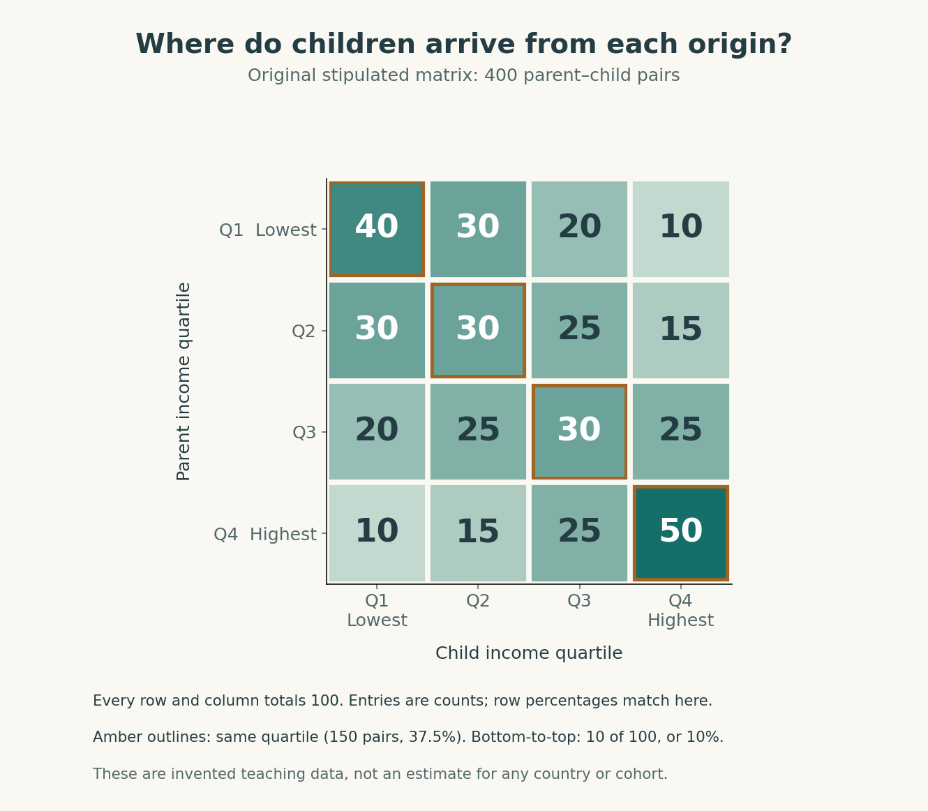
The following matrix is entirely invented for teaching. It contains four hundred parent–child pairs, divided into four parent-income quartiles and four child-income quartiles. Quartiles each contain one quarter of the relevant generation under the stipulated ranking. Every row contains one hundred pairs and every column also contains one hundred. Ties and weighting are set aside in this simplified example.

Parent's income quartile	Child Q1, lowest	Child Q2	Child Q3	Child Q4, highest	Row total
Q1, lowest	40	30	20	10	100
Q2	30	30	25	15	100
Q3	20	25	30	25	100
Q4, highest	10	15	25	50	100
Column total	100	100	100	100	400

Read across a row to follow children from a particular origin. Of the one hundred children whose parents were in Q1, forty are in child Q1 and ten are in child Q4. The bottom-to-top transition rate is therefore ten percent for children from the bottom parent quartile. The denominator is one hundred, not four hundred.

Read down a column to ask about origins among people at a destination. Of the one hundred children in Q4, ten have parents from Q1 and fifty have parents from Q4. In this special balanced matrix, counts can be read as both row and column percentages because the totals happen to match. That convenience should not become a habit when working with tables whose margins differ.

Summaries answer different questions about the same matrix

The diagonal contains forty, thirty, thirty and fifty pairs, totaling one hundred and fifty. Thus 37.5 percent remain in the same quartile. The other 250 pairs, or 62.5 percent, change quartiles. Calling this latter share “mobility” is permissible if we state the definition, but it treats a one-quartile and a three-quartile move as equally mobile.

Cells above the diagonal represent children in a higher quartile than their parents. Their counts sum to 125, or 31.25 percent of all pairs. The cells below also sum to 125. Equality of these counts is a feature of this particular matrix, not a general rule that every upward mover must be matched by exactly one downward mover.

To see why, imagine four ranks in which three people each move up one place and the fourth falls three places. The number moving up exceeds the number moving down, although the rank changes balance in magnitude. Fixed ranks constrain the distribution of positions, but they do not require equal counts of upward and downward movers. This distinction is easy to miss in a symmetrical table.

The matrix also shows persistence at both ends. A child from Q4 has a fifty-percent chance of remaining in Q4 in this invented population, compared with ten percent for a child from Q1 reaching Q4. The ratio is five to one. That is a conditional comparison of destinations given origins. It does not imply that family origin mechanically determines every child’s destination.

Independence is a useful benchmark, not a moral verdict

If child quartile were statistically independent of parent quartile in a balanced four-by-four table, each origin row would distribute twenty-five children into each destination. The bottom-to-top rate would be twenty-five percent, and the diagonal would total one hundred, or twenty-five percent of all pairs. This supplies a benchmark for comparing the association between origins and destinations.

Independence does not mean that every child has adequate resources. A society could have weak origin–destination association and severe inequality among destinations. It could also have strong persistence while ensuring a high material floor. These possibilities show why mobility and inequality should be examined together rather than treated as interchangeable measures of justice.

Nor is maximum movement automatically desirable. Forced displacement, economic collapse or widespread downward mobility can produce movement that people would reasonably dislike. A normative assessment should state whether it values opportunity independent of origins, absolute improvement, security, a reduced distance between positions or some combination. The matrix does not choose among those values.

The benchmark also depends on the categories. Four broad quartiles conceal movement within each quartile. Someone near the bottom of Q2 could move toward its top without crossing a boundary, while a small change near a cutoff could count as a quartile transition. Continuous ranks, income amounts and categorical transitions each reveal different aspects of movement.

Relative persistence can coexist with different distributions

Imagine keeping our transition matrix fixed while doubling every child's real income. The quartile transitions remain the same, provided the ordering does not change. Absolute outcomes improve, and some children who previously earned less than their parents may now earn more. A rank-based mobility measure would miss that change because it was designed to answer another question.

Alternatively, widen the distance between the highest and lowest child incomes while preserving every rank. The matrix again remains unchanged, but the stakes of reaching a particular destination become larger. This matters when evaluating a society in which opportunities to move are discussed separately from the consequences of ending at the bottom.

A complete comparison therefore needs both the transition and the distribution. The matrix answers who tends to arrive where. Income levels and dispersion help describe what those destinations provide. Household needs, public services and security may add further dimensions, as established in the first chapter. Precision means choosing the relevant set, not demanding one statistic summarize everything.

Cohorts experience different conditions

A birth cohort is a group born during a specified period. Cohorts can encounter different educational systems, labor markets, housing conditions and economic changes at similar ages. Comparing mobility across cohorts can therefore reveal changing opportunities, but it requires consistent definitions and sufficient follow-up. A younger cohort observed early in adulthood may not yet be comparable with an older cohort observed later.

Suppose a fictional study measures one cohort's income at thirty-five and another's at twenty-five. A difference could reflect cohort conditions, age or both. Calling it a generational decline would outrun the design unless those components are addressed. The same caution applies if one group is measured during a recession and another during a strong labor market.

Linking parents and children can also create selection. Some records may be missing, some people may move beyond the observed area, and some income sources may be poorly measured. The linked sample's composition matters for generalization. A large number of observations does not eliminate bias if the missing cases differ systematically from those retained.

Uncertainty is therefore broader than sampling error alone. Definitions, linkage, timing and measurement can change the interpretation even when a numerical estimate is precise. A responsible account distinguishes these issues instead of treating a narrow confidence interval as proof that every design choice is unproblematic.

Temporary extremes can create apparent movement

Suppose a parent's income is measured during an unusually poor year, placing the family in the bottom observed group. The child's income is measured during an ordinary year. Part of the apparent improvement may reflect the parent's temporary disturbance rather than a durable change in the family's economic position. The problem becomes especially relevant when researchers select origins using extreme observations.

Regression toward the mean describes a tendency for unusually extreme measurements to be followed by less extreme measurements when the extremes partly reflect temporary or random components. It does not imply that everyone is destined for the middle or that real mobility is an illusion. It identifies one process that can inflate apparent movement when a noisy observation is treated as a stable position.

Repeated observations can help distinguish persistent resources from temporary fluctuations. But averaging is not free: it requires a longer window, can exclude people with incomplete records and may conceal a meaningful shock. The right response is to explain the measurement choice and examine whether the conclusion changes under reasonable alternatives. A claim about enduring opportunity should not rest silently on a single unusually good or bad year.

This concern is distinct from changing the boundaries of quartiles. Even with identical ranking rules, measurement noise can move people across them. A transition matrix therefore inherits the strengths and weaknesses of the underlying income observations. Correctly adding its rows is necessary, but it is not a substitute for understanding how the entries were produced.

Place can select people and change their opportunities

Imagine two towns whose children later have different average incomes. One explanation is that the towns provide different opportunities during childhood. Another is that families with different resources or plans select into them. Both can operate together. Comparing the town averages alone cannot separate the contribution of the place from the characteristics of the people living there.

Moving introduces additional complications. Families may move in response to a job offer, a separation, a housing problem or a child's needs. Those events can themselves affect later outcomes. A comparison between movers and nonmovers must therefore investigate why the move occurred, when it occurred and what else changed alongside it.

The relevant geography also needs definition. A place of birth, a childhood address, a school catchment and an adult residence are not the same exposure. A study that associates adult location with adult income may be describing where people with particular opportunities end up, rather than what childhood residence caused. The location variable should match the proposed mechanism.

The next chapter uses a randomized voucher offer to investigate access to different neighborhoods. That design provides a stronger comparison for the effect of the offer, but even it does not randomize every feature of the destination or every family's decision to move. Place is a bundle of conditions, and identifying one intervention's effect does not automatically identify each component.

From a matrix to an explanatory question

Our invented matrix establishes an association between origins and destinations. It does not tell us whether transfers, education, networks, discrimination, geography or another process produced it. Those mechanisms were developed in earlier chapters precisely because a transition table cannot supply them by itself. The table defines a pattern that an explanation must address.

A useful research question might ask why children from Q1 are less likely than those from Q4 to reach the highest destination quartile. A useful next step identifies a specific pathway and evidence that could distinguish it from alternatives. Simply adding more labels to the matrix would not establish the mechanism. Nor would selecting one exceptional biography measure the pattern's prevalence.

When reading a mobility claim, reconstruct its comparison: whose origins, whose destinations, measured at what ages, in which units, over which periods and among which linked population? Then ask whether the conclusion concerns absolute improvement, relative movement or a particular social transition. Our four opening families show why those words matter. Every child can gain resources while the rank order remains intact, and the same destination distribution can accompany very different family trajectories.

Application

Calculate the matrix's bottom-to-top rate, unchanged-quartile share and upward-movement share, naming each denominator. Construct the independent benchmark and explain how it differs. Then write a 300-word comparison of the two four-family examples, separating absolute mobility, relative mobility and the child-income distribution. End with one question that the matrix cannot answer about causes.

Check your understanding: If every child's real income exceeds their parent's, must relative rank mobility be high, and does a high share changing quartiles establish that the destination distribution is equal?

Expected answer: No. Universal absolute improvement can preserve the entire rank order. Quartile changes describe origin–destination transitions, while inequality describes the distribution of resources at destinations. A society can have considerable movement and large resource differences. Both measures need their populations, periods and definitions stated explicitly.