Size changes the problem

A giant animal in a film often looks exactly like its smaller counterpart, enlarged until it towers over a street. Its legs keep the same proportions. Its surface has the same texture. Nothing visible has changed except the ruler beside it. But enlargement changes relationships within the body even when the drawing preserves every proportion. The amount to support, the surface available for exchange, and the distances between places grow at different rates.

We can reveal those changes with shapes and arithmetic before making any claim about an actual species. The resulting models will not tell us the largest possible insect, fish, or mammal. They will show what a plausible explanation of size must account for, and which assumptions need to be checked when a living animal departs from a simple enlarged copy.

Enlarge a cube before enlarging an animal

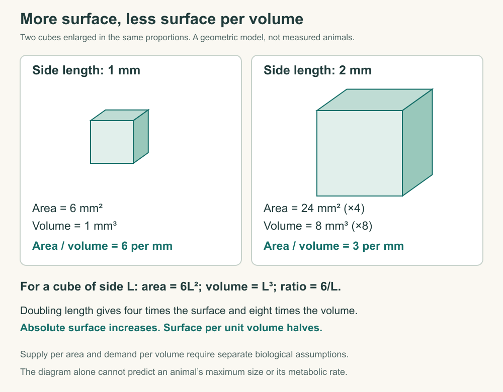
Begin with a cube whose edge is one millimeter long. Each face has an area of one square millimeter, so its six faces total six square millimeters. Its volume is one cubic millimeter. The numerical surface-area-to-volume ratio is therefore six per millimeter: six square millimeters divided by one cubic millimeter. The units matter because this is not a dimensionless fraction.

Now double every edge. Each face becomes four square millimeters, giving a total surface area of 24 square millimeters. The volume becomes eight cubic millimeters. The ratio is 24/8, or three per millimeter. The large cube has more surface in total, but less surface for each unit of volume. Saying simply that enlargement “reduces the surface area” would get the result wrong.

For an edge length L, the area is 6 × L² and the volume is L³. Their ratio is 6/L. You do not have to memorize a slogan if you can rebuild these relationships from the faces of a cube. Doubling length multiplies area by four and volume by eight; tripling length multiplies them by nine and 27.

The same powers apply when any shape is enlarged without changing its proportions. Its numerical constants may differ from the cube's, but length, area, and volume still scale by the first, second, and third powers of the enlargement factor. This kind of proportional enlargement is called isometric scaling. It is a defined comparison, not a promise about growth in a living animal.

Turn the geometry into a stated biological model

To connect the cube to an animal, add assumptions deliberately. Suppose each unit of volume contains the same amount of living tissue with the same demand for a particular resource per minute. Suppose each unit of exposed surface can transfer the same amount of that resource per minute. Under those assumptions, demand follows volume while transfer capacity follows area.

Give the small cube six units of transfer capacity per minute and one unit of demand. Its capacity is six times its demand. After doubling all lengths, the corresponding values become 24 units of capacity and eight of demand. The ratio falls to three. The larger model still has excess capacity in this invented example. A reduced ratio does not automatically mean failure.

If the small model instead began with capacity exactly equal to demand, the same enlargement would create a mismatch. The conclusion depends on the starting margin as well as the scaling powers. That is why a surface-to-volume calculation cannot supply a universal size threshold without measurements of transfer and demand. OpenStax introduces surface-to-volume relationships as a constraint on animal organization; the quantitative model here makes its extra assumptions explicit. OpenStax: animal form and function

An actual animal might alter its activity, tissue composition, exchange area, or transfer conditions as it grows. It might develop internal folds or transport routes rather than preserve geometric similarity. Those changes do not refute arithmetic. They mean that one or more assumptions connecting the arithmetic to the animal must be revised.

A longer diffusion distance changes the time scale

Surface area is only one part of an exchange problem. Material that has reached a surface may still need to travel through a medium to a receiving cell. Diffusion is effective over short distances partly because its characteristic spreading time increases strongly with distance. Doubling a distance in the same simple diffusion model requires four times the characteristic time, not twice.

For free diffusion along one dimension, the mean squared displacement is 2Dt, where D is the diffusion coefficient and t is elapsed time. The square root of that mean gives a measure of the spread. Setting this characteristic distance equal to L gives t = L²/(2D). This is a statistical spreading relationship, not an appointment at which every molecule reaches a destination. D. H. Rothman, MIT: random walks and diffusion, pages 2–5

The distinction from directed travel is substantial. In a simple constant-speed journey, twice the distance takes twice the time. Diffusing molecules repeatedly change direction; their path length is not the same as their net displacement. A fast-moving molecule can travel a long accumulated path while remaining relatively close to where it began.

We use the one-dimensional model to isolate the distance relationship. Boundaries, chemical reactions, directed flow, and different materials can change the actual problem. A real cell's supply cannot be inferred from a distance alone. The formula provides a comparison under named conditions, and it makes shortening the final distance a concrete physical strategy rather than a vague statement that thin tissues are “efficient.”

Work a diffusion comparison with consistent units

Choose an illustrative diffusion coefficient of 0.002 square millimeters per second. This is an assigned value for the calculation, not a measured coefficient for every tissue or for an identified molecule in this course. At a characteristic distance of 0.01 millimeter, squaring the distance gives 0.0001 square millimeter. Divide by twice the coefficient, 0.004 square millimeter per second, to obtain 0.025 second.

Increase the distance tenfold to 0.1 millimeter. The square is now 0.01 square millimeter, and the characteristic time is 2.5 seconds. At one millimeter, it is 250 seconds. Each tenfold distance increase has multiplied the time by one hundred. The changing times follow the squared distances; we have kept the diffusion coefficient fixed throughout.

Do not read the one-millimeter result as a guarantee that a tissue can wait 250 seconds for its next supply. The calculation does not include consumption, an exchange surface, binding, or a specified concentration requirement. It describes spreading under an idealization. Predicting how much oxygen reaches a consuming cell would require a supply-and-consumption model with those additional conditions.

The calculation nevertheless improves a body diagram. If its arrow spans a long distance and is labeled only “diffusion,” ask whether the proposed route has been justified. If fluid flow covers most of the distance before a short final exchange, show the two steps separately. A transport system does not abolish diffusion; it can place replenished material closer to the point of use.

Change shape without changing volume

Two bodies can have the same volume and different exchange geometry. A cube with ten-millimeter edges has a volume of 1,000 cubic millimeters and an area of 600 square millimeters. Reshape that volume into a rectangular block one millimeter thick, twenty millimeters wide, and fifty millimeters long. Its volume remains 1,000 cubic millimeters.

The thin block's area is twice the sum of the three distinct face areas: 2 × (20 + 50 + 1,000), or 2,140 square millimeters. It has more than three times the cube's external area. Its center is also only half a millimeter from the nearest broad face, compared with five millimeters from the nearest face in the cube. Reshaping has changed area and distance together.

If all faces were equally accessible exchange surfaces and all other relevant conditions matched, that shorter center-to-surface distance would correspond to one-hundredth the diffusion time in the same simple distance model. It would not establish one hundred times the whole body's resource supply. Area, gradients, consumption, and boundary properties still enter the supply problem in their own ways.

This imaginary block explains what to look for in a thin or flattened body. It does not show that all flattened animals share the same physiology. A living surface can be covered, folded, damaged, or poorly supplied with fresh external medium. The visible outline helps formulate questions about exchange; it cannot answer them without knowing which parts of the outline actually participate.

Folding helps only when the surface can work

An internal fold can add area without requiring the whole animal to become a broad sheet. But new area must be connected to the relevant supplies and destinations. Picture an accordion-shaped sheet immersed in still liquid. If adjacent folds nearly touch, some regions may exchange with a small pocket whose composition changes rapidly. Counting every folded square millimeter as equally supplied could exaggerate its contribution.

Now imagine the same folds with a maintained flow past their exposed sides and a transport route close behind them. The arrangement changes how material arrives, crosses, and leaves. The useful explanation is the linked route, not the fold alone. Area is available geometry; transfer is a process that depends on the conditions across that geometry.

The two faces of a thin barrier also need different descriptions. One may face an environmental medium; the other may face internal transport fluid. Increasing flow on the first side will have limited value if the second side cannot carry material away or if the barrier itself is strongly limiting. A response to one intervention helps identify where the important resistance lies.

This is why anatomical photographs need functional questions beside them. A richly branched structure looks impressive, but the image may not show its permeability, thickness, supply, or demand. To explain its operation, add those missing relationships. Detailed animal courses will use identified exchange structures rather than treating every branch or fold as evidence of the same mechanism.

Supporting a larger body is another scaling problem

Consider a simplified solid support carrying a load along its length. Average compressive stress is the force divided by the relevant cross-sectional area. Stress describes how a force is distributed; it is distinct from the resulting deformation and from the material's failure limit. OpenStax: stress, strain, and elastic modulus

Suppose a geometrically enlarged model has twice every length and the same density. Its mass, and therefore its weight under the same gravity, rises eightfold. A proportionally enlarged support has four times the cross-sectional area. If the load arrangement remains equivalent, the average stress from the weight doubles: eight divided by four is two. A bigger support can experience greater stress despite looking proportionally just as sturdy.

Use invented numbers to check the reasoning. A ten-newton load acting across ten square millimeters produces one newton per square millimeter. The enlarged comparison has eighty newtons across forty square millimeters, giving two newtons per square millimeter. Whether either support fails cannot be decided without information about material, shape, loading, and failure behavior.

A walking animal also produces changing forces and bending moments; it is not a motionless weight on a straight column. Posture, speed, limb arrangement, and tissue properties matter. The simple calculation therefore identifies a demand that proportional enlargement changes. It does not prove that large animals cannot exist or that every limb must follow one scaling rule.

Use scaling to locate the next question

Isometric scaling provides a comparison against which actual differences become visible. If a growing animal changes proportion, the comparison is no longer a simple enlarged copy. The broader study of how biological measurements change with size is called allometry. Establishing an actual scaling relationship requires data, an appropriate comparison, and attention to what the measurements represent.

Comparing stages of one species asks a different question from comparing adults of many species. The first follows development under its conditions. The second mixes size with different histories, environments, and body arrangements. A straight line through one kind of comparison should not be transferred silently to the other. The axes may have the same labels while the biological explanation differs.

For our hypothetical enlargement, write the consequences in separate rows: area rises fourfold, volume rises eightfold, a corresponding diffusion distance doubles, and its characteristic diffusion time rises fourfold. Under the specified weight-and-support assumptions, average support stress doubles. These are linked consequences of one geometric change, but each belongs to a different physical account.

A strong explanation then asks which consequence matters for the animal under study. Is exchange limiting at the activity being considered? Is the relevant distance actually enlarged? Has the support arrangement changed? Those questions turn the cube into a tool for investigation. They also protect us from mistaking an elegant ratio for a complete account of a living body.

Application

Enlarge and audit

Triple every length of the one-millimeter cube. Calculate total surface area, volume, and surface-area-to-volume ratio with units. Under the stated proportional support model, calculate the change in average stress. Explain why none of these results alone gives the maximum size of an animal.

Shorten the final route

Keep the illustrative diffusion coefficient at 0.002 square millimeters per second. Compare characteristic distances of 0.2 and 0.05 millimeter. Calculate both spreading times, then explain what the comparison does and does not establish about a consuming tissue.

Model interpretation

The enlarged cube has an area of 54 square millimeters and a volume of 27 cubic millimeters. Its ratio is two per millimeter. Area has risen ninefold and volume 27-fold. With equivalent loading, unchanged density and gravity, and proportionally enlarged support, average stress rises by 27/9, or threefold. Actual failure requires material and loading information; exchange sufficiency requires supply and demand information.

The first diffusion time is 0.04/0.004 = 10 seconds. The second is 0.0025/0.004 = 0.625 second. Reducing the characteristic distance fourfold reduces the time sixteenfold in this model. These are statistical spreading comparisons, not exact arrival times or measured rates of oxygen delivery. A tissue account also needs its boundaries, gradients, flow, and consumption.